Summary
- Since the summer of last year, the Hedgewise Momentum framework has experienced a period of significant drawdown and underperformance compared to the S&P 500
- Though this raises many reasonable questions about its efficacy, such periods are quite consistent with the strategy underpinnings and almost guaranteed to occur an average of twice per decade
- To understand this, it is useful to deconstruct "Momentum", which is really just an advanced stop-loss strategy. Such a framework is subject to periods of underperformance despite significant evidence that it provides superior long-term risk-adjusted returns
- Looking forward, the outlook remains excellent, but not because of any "timing" ability or keen insight about the market, but rather because the framework persistently shifts the odds in your favor
Introduction: The Trouble with Intuition
One of the persistent challenges of running a quantitative investment framework is dealing with periods of underperformance. Since the premise of any strategy is to drive superior long-term gains with less overall risk, it may feel like underperformance indicates a failure and suggests that perhaps the strategy has become less effective.
The problem with this intuition is that quantitative frameworks largely function by shifting your odds to a different set of risks than traditional passive benchmarks like the S&P 500. For example, Risk Parity is more vulnerable to issues with cross-asset performance and correlation, and "factor" investing is more vulnerable to various macroeconomic conditions and market microstructure. Even if, over long periods of time, such risks are less persistent and damaging compared to the risks facing the S&P 500, they are still bound to manifest occasionally, and this will naturally drive periods of underperformance.
As a simple example, imagine that the S&P 500 is a bit like a coin with a 60% chance of landing on heads, and a framework is like a completely separate coin with a 65% chance of landing on heads. Given 100 flips, the advantages of the framework will seem objectively obvious. But on any given flip, there's a pretty high chance that the S&P 500 lands heads and the framework lands tails. Despite the odds that the framework will consistently perform better, there will be frequent short-term exceptions.
As with any probability, the only way to converge towards the 'true' odds is to ignore each individual datapoint and keep playing for a relatively long time. Yet, as investors in the midst of losing money, it is natural to fear that the odds have changed, and to consider whether simpler passive strategies would be a better choice. By clearly deconstructing the elements of the Momentum strategy, this article will highlight exactly what has driven its historically superior returns and why this should continue to drive confidence moving forward.
Back to Basics: What is Momentum?
Broadly, the term "Momentum" is used to refer to investment strategies that assume certain trends tend to continue over time. For example, some trend-following frameworks assume that the best-performing stocks over the past year will continue to outperform, or if stocks have done badly recently, they will go on to do even worse. There is a great ongoing debate about how and why a factor like momentum would have such predictive power.
I believe the idea that trend-following strategies have significant predictive ability is simply not credible. That said, I also believe that using momentum as a framework can significantly improve your risk-adjusted returns. How can this be?
This is far easier to explain if you consider that a simple stop-loss mechanism - a rule to sell something after incurring a certain amount of loss - is functionally the same as momentum. If things keep going up, you hold on. If they go down a certain amount, you sell. It would be absurd to argue that such a trigger had any predictive power. Rather, this is more clearly a simple form of risk management, and the relative success of such a framework will be easy to predict. If an asset keeps going down, you avoid losses. If it doesn't, you incur some cost of selling and re-entering (called a "whipsaw" effect). The main benefit of this framework would be to minimize the size of your worst losses, presuming that the worst-case impact of whipsaws should be less severe than the worst-case impact of market crashes.
In terms of efficient market theory, this makes sense. Investors are always considering risk and reward, with the expectation of paying a discount for an underlying asset in the present in order to achieve a positive return in the future. Efficient markets should usually go up, and they shouldn't remain at the same level for very long. Thus, whipsaws shouldn't happen very often. Given that, it's believable that the drawdowns incurred during market crashes may be steeper than those incurred during whipsaws.
The entire validity of 'momentum' becomes a simple trade-off of probabilities. You aren't expecting to predict anything with accuracy, and you aren't trying to figure out whether a whipsaw or a crash is going to occur. You are simply shifting around the risks of your portfolio.
Simple enough: let's make this our hypothesis, and set-up some experiments to test it.
Testing the Hypothesis: First Experiments and Mechanics
To test our hypothesis, we'll first set-up three dead simple strategies that follow one rule: if the S&P 500 hits a certain level of drawdown, sell. Otherwise, invest. Upfront, realize that this first iteration cannot possibly beat the return of the S&P 500 unless you stopped the simulation right in the middle of a big crash. But it's still a useful first experiment to understand some of the mechanics.
We'll set-up three loss triggers to explore: -10%, -15%, and -20%. The goal is to test whether the hypothesis holds up with all of these levels, since they are all consistent with the broad idea.
Performance of Stop-Loss Strategies vs. S&P 500, 1950 to Today
| Annual Return | Max Loss | |
|---|---|---|
| S&P 500 | 11.15% | -54.98% |
| -10% Stop Loss | 8.81% | -30.77% |
| -15% Stop Loss | 9.03% | -36.55% |
| -20% Stop Loss | 9.41% | -40.33% |
Note that each of the stop-loss strategies has a substantially lower annual return, but also a lower maximum loss. This confirms the hypothesis that the worst-case 'whipsaw damage' tends to be lower than worst-case 'stock crash damage', but you may be still be surprised that a 10% stop-loss can experience a 30% drawdown. This is mechanically important to understand as it demonstrates how whipsaws function. Here's a look at one rough stretch for the 10% strategy.
Understanding the Whipsaw Effect: December 1973
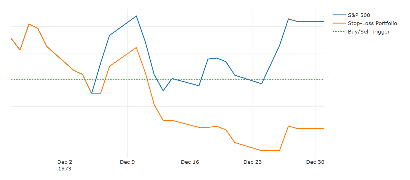
Here, the stop-loss trigger is frequently hit, and every time the portfolio liquidates. Then, the day after, stocks often recover and the portfolio buys again, but misses that days' gain. This is the whipsaw effect, which can thus accrue significant losses independent of the performance of the S&P 500. An important takeaway to highlight is that any stop-loss strategy will by definition do worse than stocks during periods where the market whipsaws, so you are likely to experience drawdowns when stocks do not, but you avoid losses when stocks crash.
While this seems scary and random, it is! But remember that's on purpose - you are actively choosing 'whipsaw crashes' over 'stock market crashes' and hypothesizing that it's still preferable.
Given the initial numbers, this doesn't seem like a clear conclusion. To enable a more equal comparison, we need to better take advantage of the stop-loss structure.
Engineering Fairer Odds
One of the substantial hidden handicaps of simple stop-loss strategies is that they will spend very long periods of time invested in nothing at all. For example, if stocks lose 40%, and take a few years to get back above a 10% net drawdown level, the strategy is 100% cash for those years. The period from 2000 to 2007 exhibits what this looks like.
Daily Stop-Loss Performance, 2000 to 2007
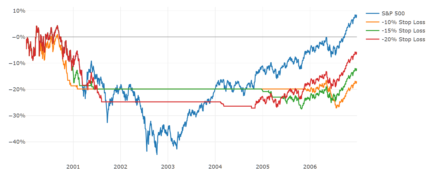
Spending this amount of time in cash is a bit of an unfair disadvantage. To correct it, we can simply choose a relatively low risk asset that is expected to accrue positive interest over these stretches. Bonds are the obvious choice, but remember that this is in no way timing bonds as the 'smart investment' when the trigger is hit. It's simply a way to deploy a positive yielding alternative when the portfolio is largely in cash. While sometimes bonds might do particularly well if markets go on to crash, they may also do poorly if markets stabilize. The stop-loss framework only cares that the net return is expected to be positive on average, especially when it is out of stocks for a significant duration of time.
If we use 10yr Treasury Bonds as a proxy, here is how it changes the performance of the 10% stop-loss strategy in the same timeframe.
Daily 10% Stop-Loss Performance Comparison, 2000 to 2007
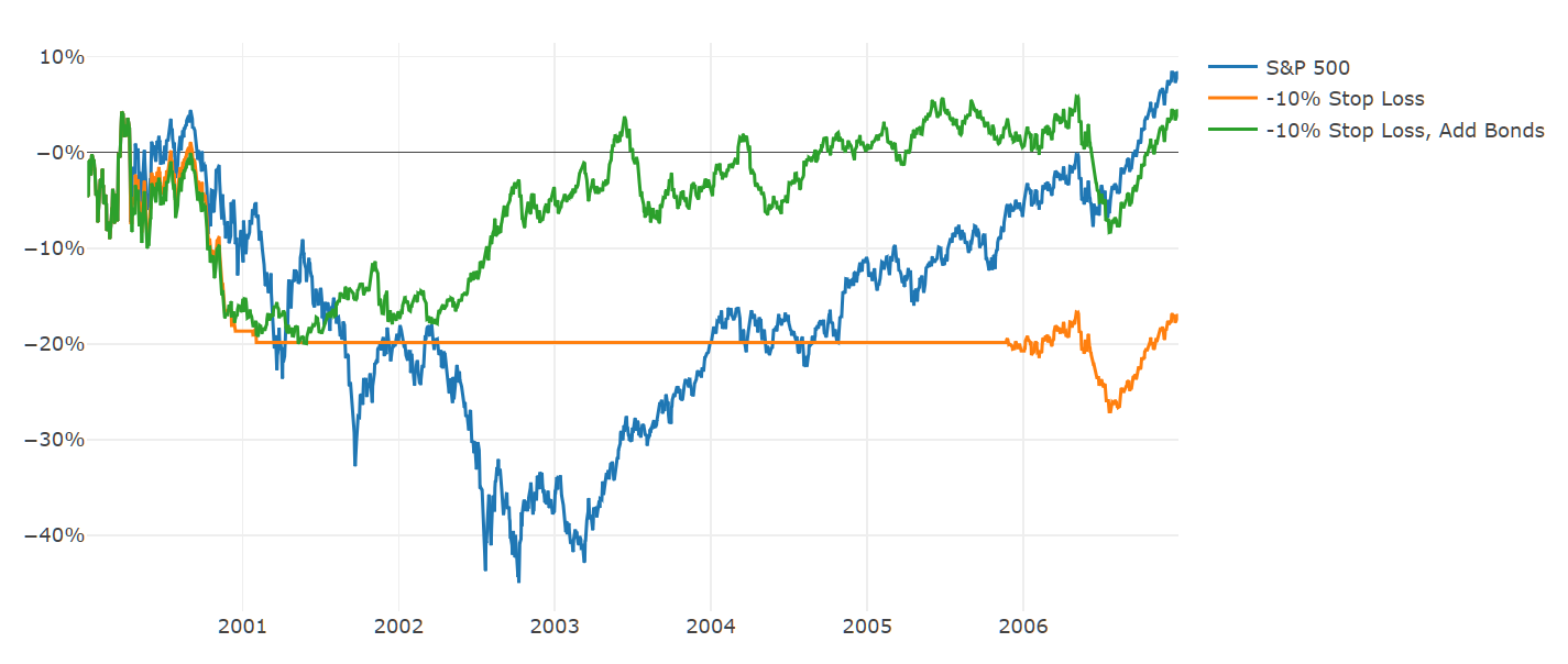
Observe that bonds significantly underperformed stocks for years beginning in 2003, but it isn't our goal to always outperform the S&P: we simply wanted to do better than cash for a stretch to avoid the stop-loss 'handicap'. It's also worth highlighting how this adjustment reduces the chances of hitting a particularly unlucky sequential drawdown, such as the cumulative impact of the whipsaws in 2001 and then subsequently in 2006.
Here's how the numbers change if we add this bond rule to each of the experimental portfolios and run it again since 1950.
Performance of Stop-Loss Strategies, Add Bonds, vs. S&P 500, 1950 to Today
| Annual Return | Max Loss | |
|---|---|---|
| S&P 500 | 11.15% | -54.98% |
| -10% Stop Loss, Add Bonds | 11.27% | -23.85% |
| -15% Stop Loss, Add Bonds | 10.72% | -26.1% |
| -20% Stop Loss, Add Bonds | 10.26% | -34.58% |
This is a pretty dramatic effect! This alone makes the 10% Stop-Loss portfolio look more compelling than the S&P 500. However, we'd prefer our hypothesis to hold up consistently across all the portfolios to demonstrate greater statistical significance, and it's very unlikely that the 10% level has some unique special power. It's also still difficult to properly evaluate the 15% and 20% levels, which exhibit both lower annual returns and lower max losses.
The Introduction of Leverage
As you can see in the tables, a buy and hold approach would have experienced a 55% drawdown. It is interesting to consider what the return would be in the stop-loss portfolios if one were willing to tolerate that level of risk. Introducing leverage provides an easy way to do just that. Since you have a built-in mechanism (the stop-loss) to help avoid large crashes, it seems sensible to also amplify your exposure. The following adds a constant 50% 'loan' to the portfolio with an assumed cost equal to the rate on 1yr Treasury Bills.
Performance of Stop-Loss Strategies, Add Bonds and 50% Leverage, vs. S&P 500, 1950 to Today
| Annual Return | Max Loss | |
|---|---|---|
| S&P 500 | 11.15% | -54.98% |
| -10% Stop Loss, Add Bonds, 150% | 14.36% | -35.57% |
| -15% Stop Loss, Add Bonds, 150% | 13.43% | -41.45% |
| -20% Stop Loss, Add Bonds, 150% | 12.6% | -52.42% |
Now our hypothesis is beginning to look more convincing: every portfolio outperforms the S&P 500 without increasing your maximum loss, yet all of these portfolios still underperform the S&P 500 for lengthy periods of time. Mechanically, this must happen every time a whipsaw occurs. The existence of these periods does not change the idea that your odds were consistently improved over the long-run.
Demystifying "Momentum": Slightly Smarter Engineering
Hopefully, it is clear that all of our work thus far has little to do with secret signals or mysterious predictions. It's just plain financial engineering and probabilities. Introducing a few more intelligent tweaks will illustrate how these same principles apply to nearly all forms of "Momentum" you may hear about in the marketplace.
Some of the most common momentum "metrics" involve the use of moving averages and trailing returns (for example, sell stocks when they fall below their 200day moving average, buy otherwise). These are little more than advanced forms of 'stop-loss' strategies. For example, here's a comparison of a simple -10% stop-loss sell trigger, a 100day trailing return sell trigger, and a 1yr moving average sell trigger.
Stop-Loss Trigger vs. Trailing Return Trigger vs. Moving Average Trigger
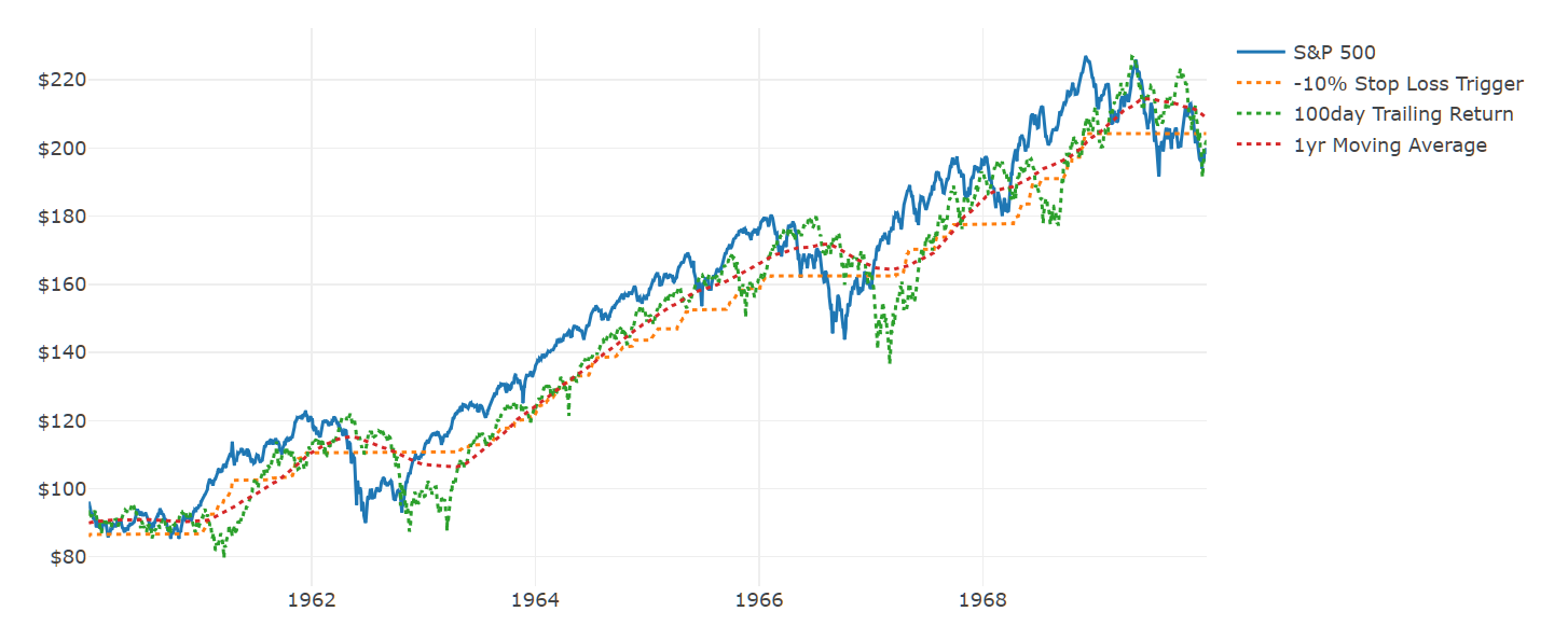
Notice how closely the dotted-lines often cluster; for a great majority of the time, there's no functional difference between them. The main advantage of the 'advanced' metrics are they build in one important and convenient heuristic: they allow for a re-entry point to equities after a big crash.
Recall in one of our earlier examples how the stop-loss strategies remain can remain in bonds for years at a time, and thus never take advantage of potentially 'cheaper' equity prices. Metrics like trailing returns and moving averages provide a convenient mechanism to re-enter stocks if prices have fallen significantly. To illustrate, here's how the various triggers moved around during the recession in the mid-1970s.
Stop-Loss Trigger vs. Trailing Return Trigger vs. Moving Average Trigger, 1970s
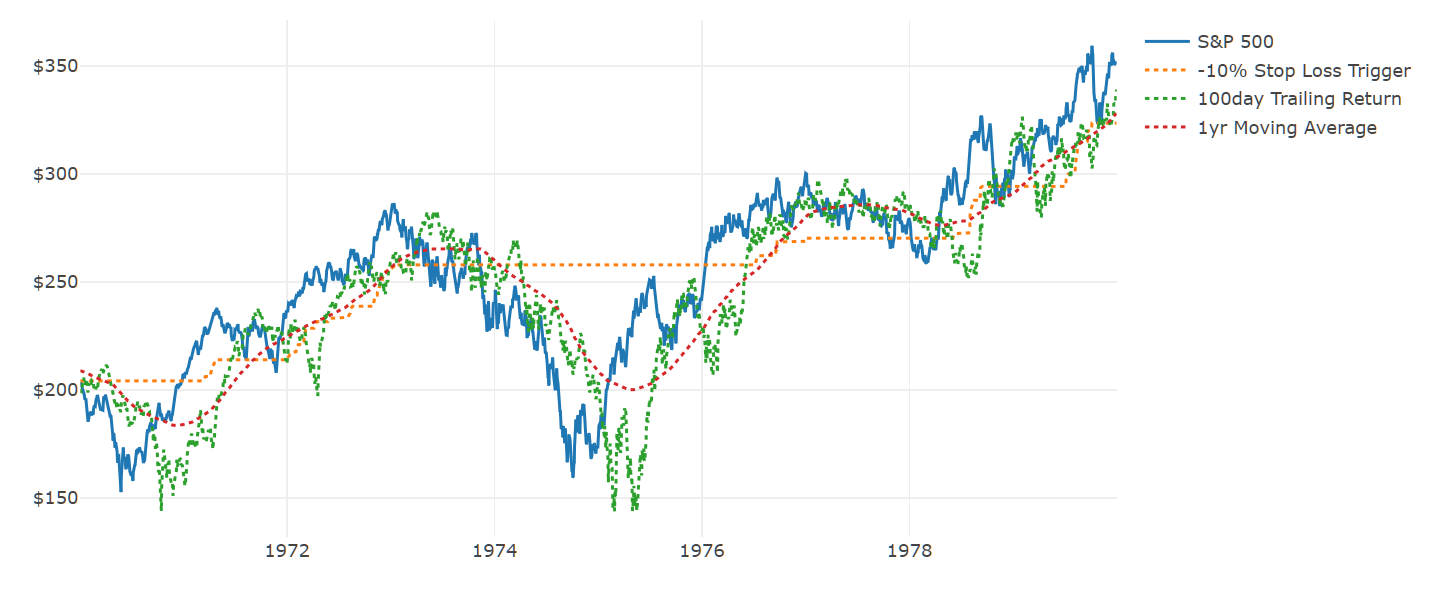
Allowing for a lower re-entry point to equities drives some significant potential extra upside, which can be seen by translating these triggers into the correlating actual performance.
Stop-Loss vs. Trailing Return vs. Moving Average Performance, 1970s
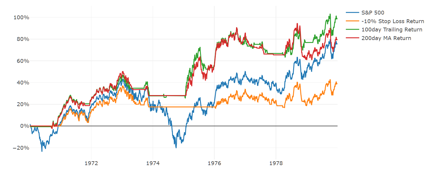
Note that the strategies only really separate as the recovery ensues between 1975 and 1976. Conversely, it's not as if the momentum metrics are immune to whipsawing, and they'll have other periods of churn where they look worse, as they did at the end of the 70s.
Stop-Loss vs. Trailing Return vs. Moving Average Performance , 1976 to 1980
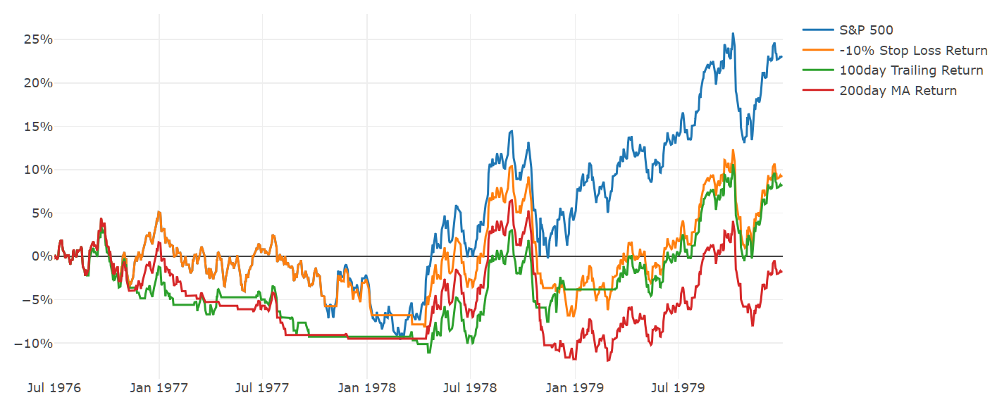
This illustrates again that whipsaws will occur somewhat randomly around whichever level you happen to choose. That said, it seems perfectly logical that you might achieve some extra upside by allowing for re-entry points after significant equity losses, and these sorts of metrics are a convenient means of doing so. We can return to our identical framework from above to see whether this proves true, starting with the simple case of no leverage, but using bonds rather than cash whenever the triggers hit.
Stop-Loss vs. Trailing Return vs. Moving Average Performance, Add Bonds, 1950 to Today
| Annual Return | Max Loss | |
|---|---|---|
| S&P 500 | 11.15% | -54.98% |
| -10% Stop Loss Return, Add Bonds | 11.27% | -23.85% |
| 100day Trailing Return, Add Bonds | 11.76% | -25.47% |
| 200day MA Return, Add Bonds | 12.53% | -20.86% |
This seems about right. If we then inject 50% leverage, all the better.
Stop-Loss vs. Trailing Return vs. Moving Average Performance, Add Bonds and 50% Leverage Performance, 1950 to Today
| Annual Return | Max Loss | |
|---|---|---|
| S&P 500 | 11.15% | -54.98% |
| -10% Stop Loss Return, Add Bonds, 150% | 14.36% | -35.57% |
| 100day Trailing Return, Add Bonds, 150% | 15.15% | -37.32% |
| 200day MA Return, Add Bonds, 150% | 16.32% | -29.97% |
These numbers are already starting to look pretty fantastic, and in some ways, it's easy to see why moving averages might appear to be 'powerful indicators'. But this analysis clearly dispels the notion of any predictive power, and each individual case of hitting a 'trigger' means nothing at all. This outperformance is driven solely through a mix of financial engineering and long-term probability. Thus, ironically, indicators like moving averages can be plenty useful despite meaning nothing at all!
Pressure Testing: Picking a Level, Dealing with Noise
One of the very tricky elements of this framework is that you have to choose a particular trigger, and that will seem like a big deal. Should it be a moving average? A trailing return? How do you choose the best one? What if you choose wrong?
The problem with this is that we've already established that this is not a market timing strategy and that whipsaws around any particular level are random and will occur. On the one hand, that means it shouldn't really matter which trigger you choose. On the other hand, it also means that there's a really, really high chance that some other trigger will be doing better than yours, but even so, there's no reason to think you should use that one instead.
To understand this better, let's expand the scope of our triggers to include many moving averages and trailing returns. If our theory is correct, all of them should exhibit similar performance profiles, though there will also be substantial noise given the randomness of whipsaws.
Various Daily Momentum Metrics Performance, Add Bonds and 50% Leverage, 1950 to Today
| Annual Return | Max Loss | |
|---|---|---|
| S&P 500 | 11.15% | -54.98% |
| 100day Return, Add Bonds, 150% | 15.15% | -37.32% |
| 200day Return, Add Bonds, 150% | 14.03% | -52.7% |
| 3mth Return, Add Bonds, 150% | 15.18% | -41.49% |
| 6mth Return, Add Bonds, 150% | 16.46% | -46.7% |
| 1yr Return, Add Bonds, 150% | 14.44% | -51.45% |
| 50day MA, Add Bonds, 150% | 15.63% | -35.44% |
| 100day MA, Add Bonds, 150% | 15.96% | -53.52% |
| 200day MA, Add Bonds, 150% | 16.32% | -29.97% |
| 6mth MA, Add Bonds, 150% | 15.73% | -53.95% |
| 1yr MA, Add Bonds, 150% | 16.28% | -40.27% |
In another fun twist, this also holds up in the same way if you make all of these monthly triggers - meaning you only trade on them once a month, rather than daily.
Various Monthly Momentum Metrics Performance, Add Bonds and 50% Leverage Performance, 1950 to Today
| Annual Return | Max Loss | |
|---|---|---|
| S&P 500 | 11.16% | -52.82% |
| 3mth Return, Add Bonds, 150% | 14.71% | -37.29% |
| 6mth Return, Add Bonds, 150% | 15.42% | -34.89% |
| 1yr Return, Add Bonds, 150% | 13.9% | -43.39% |
| 3mth MA, Add Bonds, 150% | 13.0% | -38.37% |
| 6mth MA, Add Bonds, 150% | 15.43% | -38.1% |
| 10mth MA, Add Bonds, 150% | 15.9% | -33.81% |
| 12mth MA, Add Bonds, 150% | 15.61% | -36.97% |
It is natural to gravitate towards the better performing raw numbers, but a different view of the rolling trailing ten year cumulative performance of a few of these strategies helps to show the powerful effect of randomness.
10 Year Trailing Performance
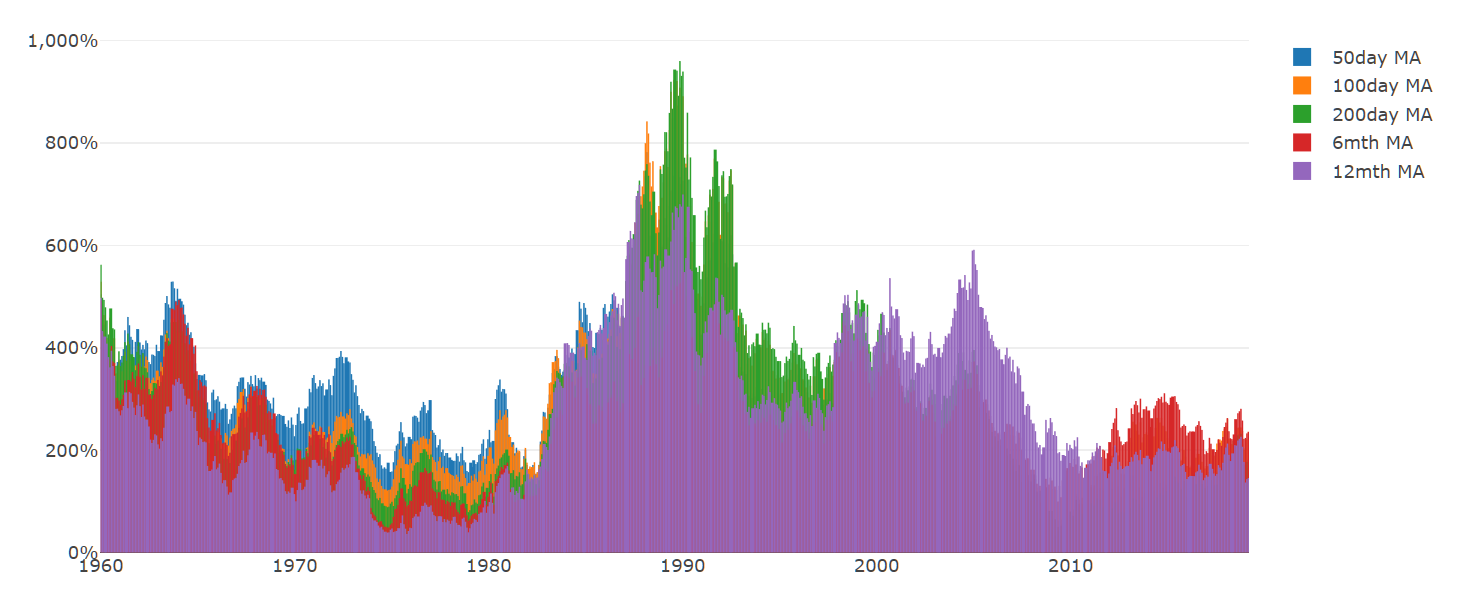
Every one of these strategies has some good decades and some bad ones, with no discernable pattern. When you look at the summary numbers, the 200day MA stands out as having one of the top returns, but that's only because of one random spike in the early 90s. Outside of that, there's nothing to suggest that it is somehow superior.
The most productive way to approach this choice is to pick a metric at random with confidence that you have an incredibly high chance of beating the S&P 500 over the long-term. It will be pure luck whether you wind up with 2% or 4% outperformance, and that's perfectly okay.
Sorting Through the Short-Term
This story sounds convincing when you are looking at ten-year time horizons, but the implications for the short-term can be quite challenging. When the strategy sells stocks, it will feel like you are trying to time a downturn (though you aren't). When you get hit by a whipsaw, it will feel like your strategy has failed (though it hasn't). Looking forward, you face an unavoidable element of randomness that will determine how well you perform in the future.
The key to sorting through this is to constantly orient your perspective to this very moment: right now, this year, does the framework give me better odds than the S&P 500?
One nice visualization to answer this is the 1yr trailing returns of one of the stop-loss strategies compared to the S&P 500. The 100day MA metric is selected randomly for comparison, but note that every metric from the prior tables returns similar looking results.
1yr Trailing Performance, 100day MA Strategy vs. S&P 500
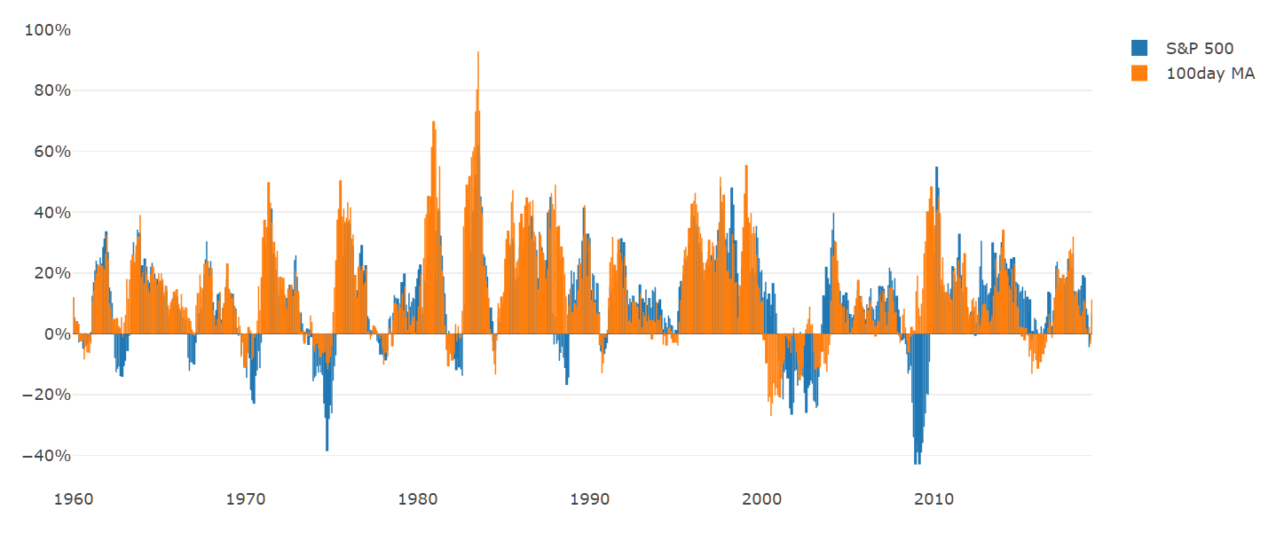
What jumps out immediately is that, on net, your returns are higher, more stable, and less prone to severe drawdowns. But you'll still have bad stretches and they'll often happen independently of equities.
The question is, given we can't know what the next 12 months will bring, which set of possible outcomes would you choose?
The Hedgewise Framework
At various point throughout this article, if you've thought "I wonder if you could tweak these rules in certain ways to make them even better", I have great news for you: the answer is yes, and this is what Hedgewise does! There are a couple of additions that are especially useful, such as layering on diversification across assets, and employing differing levels of exposure based on the environment.
While Hedgewise has abundant theory and research to suggest these are effective modifications, it's crucial to understand that the goal is still never to time the market. Instead, it's useful to return to the probabilities: imagine the simple momentum metrics above have about a 30% chance of hitting a whipsaw in any given year, and Hedgewise manages to reduce that probability to 20%. Even given this dramatic improvement, you still fully expect two whipsaws per decade!
By accepting whipsaws as inevitable in any form of this broad framework, it becomes easier to shift focus towards probabilities and long-term returns (rather than on each individual whipsaw and whether it could have been avoided). Using this lens, let's take a look at the relative effectiveness of Hedgewise methods.
First, let's examine the same prior graph of 10yr trailing performance across various Momentum metrics, but add in the specific Hedgewise "Momentum Max" framework as well. The other metrics are still assuming that you have added bonds and 50% leverage.
10yr Trailing Performance, Hedgewise vs. Prior Momentum Metrics
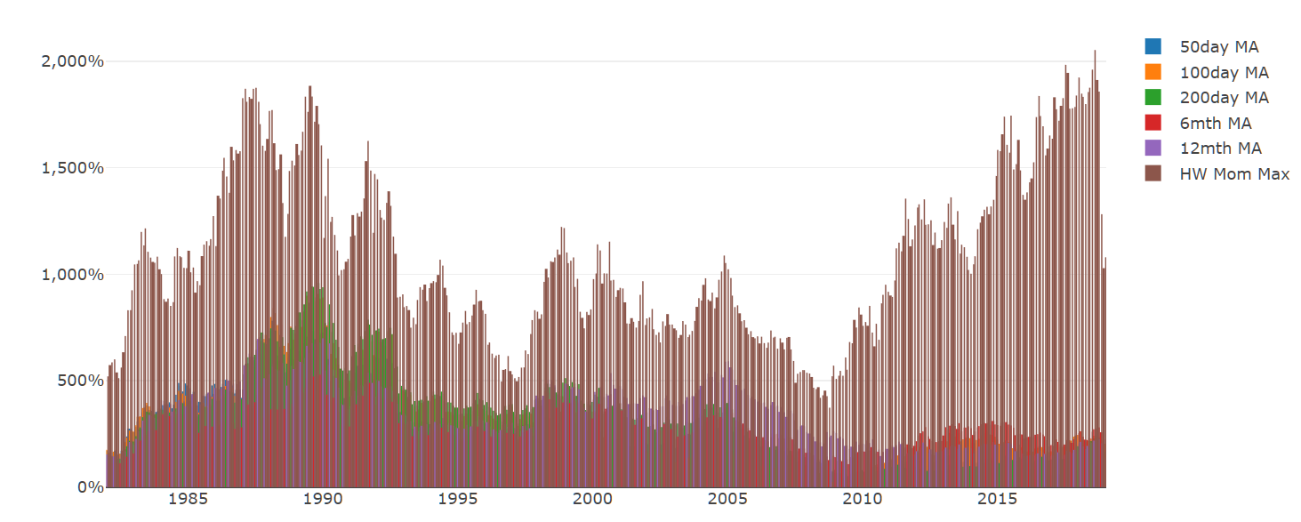
The Hedgewise Momentum Max portfolio is the brown bar, and there is not a single datapoint in which it has trailed the simpler momentum metrics. However, there is still a significant ebb and flow to the absolute performance, which naturally exists for the reasons already discussed.
Let's zoom in to look at the shorter 1yr trailing performance. This is the identical prior graph examining the performance of the 100day MA strategy, including bonds and 50% leverage, against the S&P 500. The trailing 1yr performance of the Hedgewise Momentum Max model has been added for comparison.
1yr Trailing Performance, Hedgewise Momentum Max vs. 100day MA vs. S&P 500
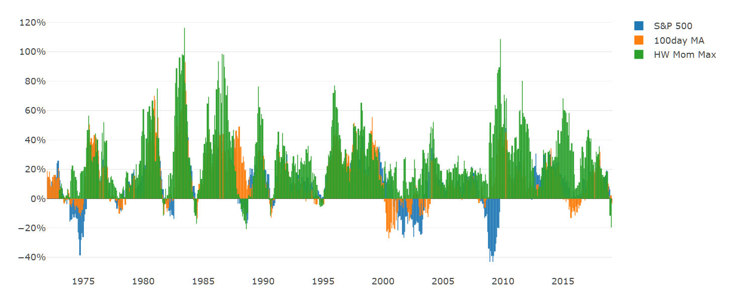
While the Hedgewise model drives consistently superior returns and a lower probability of loss, the natural variation still results in periods where it looks bad compared to simpler momentum metrics as well as the S&P 500. This is not a sign that anything is wrong, but rather an inevitability of our odds-based framework.
Conclusion: Reflections on Current Performance
Bringing all of this theory back together with our current reality, it's difficult to defend a drawdown of a Momentum framework in isolation when there's such a purposeful element of randomness involved. That said, I'd say it's pretty easy to see why the market conditions of the past few months are fairly exceptional: the jaw-dropping drops in December remain difficult for anyone to fully explain, especially given the enormous reversal in January. Part of this can be attributed to the Fed making one of the most dramatic and speedy policy U-turns in history - which on its own is extremely unique! The point being that it takes a rare combination of factors to drive a whipsaw, and that's precisely why momentum frameworks have worked so well and will likely continue to work.
It's also really important to focus on the performance of the Hedgewise strategy outside of the period of whipsaw, since the whole idea is that it's a great bet so long as it's not whipsawing. In March alone, Momentum Max is currently +6.5%, compared to a 0.9% gain in stocks. From the launch of the strategy in November 2016 through September 2018, Momentum Max also beat equities by 10%. These are relatively common outcomes because markets are generally efficient.
That said, it's also not like the returns are driven by anything dramatic: you primarily make money in the momentum framework because stocks go up (and bonds, to a lesser extent). This is still the bet you are making, same as if you were in a purely passive index. Will another whipsaw occur? Probably! But the whole beauty of the framework is that you don't have to predict that, or try to avoid it, because it hasn't mattered over the long-run. You just have to sit tight and keep playing the game long enough to see.
Disclosure
This information does not constitute investment advice or an offer to invest or to provide management services and is subject to correction, completion and amendment without notice. Hedgewise makes no warranties and is not responsible for your use of this information or for any errors or inaccuracies resulting from your use. Hedgewise may recommend some of the investments mentioned in this article for use in its clients' portfolios. Past performance is no indicator or guarantee of future results. Investing involves risk, including the risk of loss. All performance data shown prior to the inception of each Hedgewise framework (Risk Parity in October 2014, Momentum in November 2016) is based on a hypothetical model and there is no guarantee that such performance could have been achieved in a live portfolio, which would have been affected by material factors including market liquidity, bid-ask spreads, intraday price fluctuations, instrument availability, and interest rates. Model performance data is based on publicly available index or asset price information and all dividend or coupon payments are included and assumed to be reinvested monthly. Hedgewise products have substantially different levels of volatility and exposure to separate risk factors, such as commodity prices and the use of leverage via derivatives, compared to traditional benchmarks like the S&P 500. Any comparisons to benchmarks are provided as a generic baseline for a long-term investment portfolio and do not suggest that Hedgewise products will exhibit similar characteristics. When live client data is shown, it includes all fees, commissions, and other expenses incurred during management. Only performance figures from the earliest live client accounts available or from a composite average of all client accounts are used. Other accounts managed by Hedgewise will have performed slightly differently than the numbers shown for a variety of reasons, though all accounts are managed according to the same underlying strategy model. Hedgewise relies on sophisticated algorithms which present technological risk, including data availability, system uptime and speed, coding errors, and reliance on third party vendors.
